Evaluating the Models
Note: This is earlier work I did (last winter/spring) so some info may seem dated at time of posting. I’ve used data files current to then.
Last post we predicted the results of the remainder of the season. It’s exciting to know that your favourite team might make the playoffs, but how can you trust the model? We haven’t performed any validation so far. Maybe all the work we’ve done is a worse predictor than a 50/50 split of winners? Lets dive in and find out.
We’ll start by evaluating the models for ‘RPS’ (Rank Probability Score). There’s a great discussion of why this is important by Anthony Constantinou that you can read here (pdf). The great thing is, the RPS calculation is already available in R from the verification package.
library(verification) #This requires the latest version of R to properly load.The RPS formula takes a matrix of probabilities and a result, and returns the score based on how close the model was. For example, if team A (away) was given a 0.6 chance of winning, team B (home) a 0.25, and a draw of 0.15, then the probability set is {A,D,H} = {0.6,0.15,0.25}. If Team B wins, then the result is 3, the third column. The formula for RPS is:
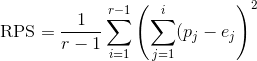
where: r is the number of potential outcomes (in our case, 3), p j is the pobability of outcome at position j, and e j is the actual outcome at that position.
Our example looks as this:
 |
 |
RPS |
|---|---|---|
| {0.6,0.75(,1)} | {0,0(,1)} | 0.46125 |
Normally, the summation sets don’t include the 1, that value is implied.
A smaller RPS value is better, so when we get a ‘home’ win with RPS = 0.46125, or an away win with RPS = 0.11125, we can say that the model ‘performed better’ with the prediction of an away win. There are more examples of performance in the above linked paper by Constantinou.
To evaluate each model, let’s compare the results of 2014-2015 season to our predictions. We’ll start with training the model with all the games up to December 31 (approximately the first half of the season), and compare the predicted results to the actuals from then to the end of the season. We can experimentally determine a better value for ξ (see the time-weight dependance post) than the 0.005 we’ve tossed around.
To start, let’s build a 2015 testing data (a schedule), 2015 training data, 2015 known results, and 2005-2014 data for longer predictions.
data_2015 <- nhl2015 <- getAndPrepAllData(year_list = c(2015))
train_2015 <- data_2015[data_2015$Date <= as.Date("2014-12-31"), ]
train_long <- getAndPrepAllData(year_list = c(2006:2014))
train_long <- rbind(train_long, train_2015)

test_schedule <- data_2015[data_2015$Date > as.Date("2014-12-31"), ]
test_schedule$HG <- test_schedule$AG <- test_schedule$OT.SO <- test_schedule$OT.Win <- ""

test_results <- data_2015[data_2015$Date > as.Date("2014-12-31"), ]
# Get A,D,H = 1,2,3 results
test_results$Result <- ifelse(test_results$OT.SO != "", 2, ifelse(test_results$AG >
    test_results$HG, 1, 3))
test_results <- as.vector(subset(test_results, select = c(Result)))
Now, we can start running the optimizer on our data sets to get our Dixon-Coles parameters. Recall that these are long processes.
res_2015 <- doDCPrediction(train_2015)
res_long <- doDCPrediction(train_long)
Now with our res sets, we can evaulate the performance of each to the actual data. Instead of predicting a score, all we need to do is get the proportion of A,D,H for each game. We can recycle earlier code with a different return to get this information:
getWinProp <- function(res, home, away, maxgoal = 8) {
    attack.home <- paste("Attack", home, sep = ".")
    attack.away <- paste("Attack", away, sep = ".")
    defence.home <- paste("Defence", home, sep = ".")
    defence.away <- paste("Defence", away, sep = ".")

    # Expected goals home
    lambda <- exp(res$par["HOME"] + res$par[attack.home] + res$par[defence.away])
    # Expected goals away
    mu <- exp(res$par[attack.away] + res$par[defence.home])

    probability_matrix <- dpois(0:maxgoal, lambda) %*% t(dpois(0:maxgoal, mu))

    scaling_matrix <- matrix(tau(c(0, 1, 0, 1), c(0, 0, 1, 1), lambda, mu, res$par["RHO"]),
        nrow = 2)
    probability_matrix[1:2, 1:2] <- probability_matrix[1:2, 1:2] * scaling_matrix

    away_prob <- sum(probability_matrix[upper.tri(probability_matrix)])
    draw_prob <- sum(diag(probability_matrix))
    home_prob <- sum(probability_matrix[lower.tri(probability_matrix)])

    return(c(away_prob, draw_prob, home_prob))
}

getADHSeason <- function(schedule, res, maxgoal = 8) {
    adh_results <- data.frame(A = NA, D = NA, H = NA)
    for (game in 1:nrow(schedule)) {
        home <- as.character(schedule[game, "HomeTeam"])
        away <- as.character(schedule[game, "AwayTeam"])
        adh <- getWinProp(res, home, away, maxgoal = maxgoal)
        adh_results <- rbind(adh_results, adh)
    }
    adh_results$A <- as.numeric(adh_results$A)
    adh_results$D <- as.numeric(adh_results$D)
    adh_results$H <- as.numeric(adh_results$H)
    return(adh_results[2:nrow(adh_results), ])
}
We can get our ADH probability for the test data quite simply. We take it as a matrix to make it ready to feed into the rps function:
adh_2015 <- as.matrix(getADHSeason(test_schedule, res_2015, maxgoal = 8))
adh_all <- as.matrix(getADHSeason(test_schedule, res_long, maxgoal = 8))

rps_2015 <- rps(unlist(test_results), adh_2015)
rps_all <- rps(unlist(test_results), adh_all)
Now, lets look at the rps results to see how they compare. For 2015 only data in the model, our RPS value is 0.233542, and for all the available data, it’s 0.2334388. Not a huge difference. But, lets’ optimize the xi value by using RPS.
min_xi <- function(x, train, schedule, currentDate = Sys.Date()) {
    res <- doDCPrediction(train, xi = x, currentDate = currentDate)
    adh <- as.matrix(getADHSeason(schedule, res, maxgoal = 8))
    rps <- rps(unlist(test_results), adh)
    return(unlist(rps[1]))
}

opt_xi <- optimize(min_xi, lower = 0, upper = 0.05, train = train_2015, schedule = test_schedule,
    currentDate = as.Date("2014-12-31"))
opt_xi_long <- NULL
opt_xi_long$minimum <- 0.01914645
opt_xi_long$objective["rps"] <- 0.2407655So we see that for the 2015 data only, we get an optimal xi value of 0.0184461, with an RPS of 0.2334589. We can do optimization for the full data as well. You’ll have to believe me when I say that the optimal xi value takes a lot longer to elucidate, but it’s 0.0191464, giving us an RPS of0.2407655.
Let’s compare some more methods, to know how well this model really compares. We don’t know if this RPS value is good or bad, so let’s use some dummy data. If the home team wins every game, our odds are {0,0,1}. If we use the ‘50-50’ win method, our odds for each game are {0.5,0,0.5}. If we consider OT/SO results, we’ll have approximately {0.4,0.2,0.4} for each game. the RPS for both is calculated. One final matrix of randomly generated proportions is tested too.
rps_home <- rps(unlist(test_results), (t(matrix(c(0, 0, 1), ncol = length(unlist(test_results)),
nrow = 3))))
rps_even_no_ot <- rps(unlist(test_results), (t(matrix(c(0.5, 0, 0.5), ncol = length(unlist(test_results)),
nrow = 3))))
rps_even <- rps(unlist(test_results), (t(matrix(c(0.4, 0.2, 0.4), ncol = length(unlist(test_results)),
nrow = 3))))
randFun <- function(n) {
m <- matrix(runif(3 * n, 0, 1), ncol = 3)
m <- sweep(m, 1, rowSums(m), FUN = "/")
return(m)
}
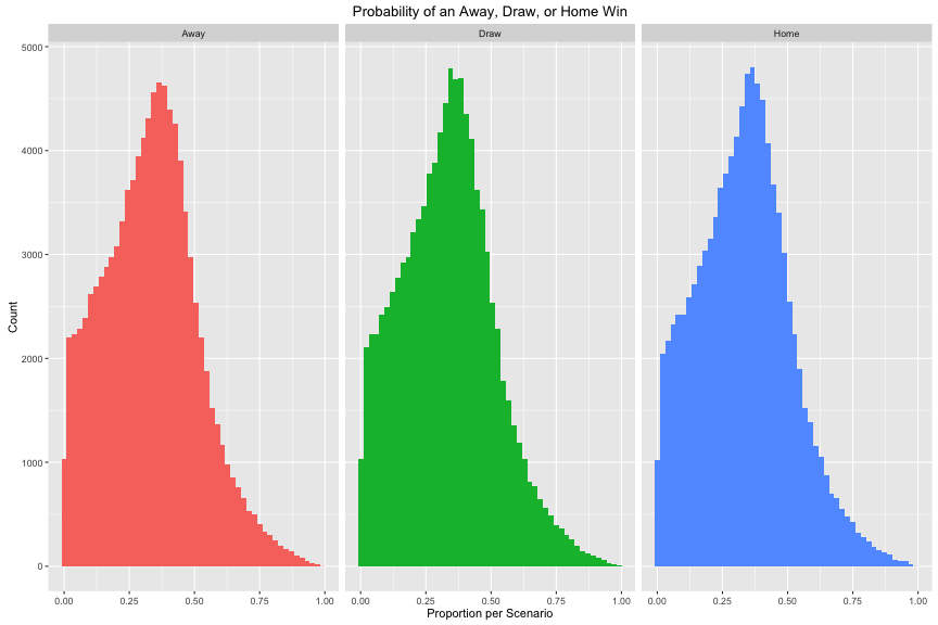
rps_rand <- rps(unlist(test_results), randFun(n = length(unlist(test_results))))The distribution of each (Away, Draw, Home) is shown in this plot:
This gives us the following results:
| Method | RPS |
|---|---|
| Short Training | 0.233542 |
| Long Training | 0.2334388 |
| Short Training (time weighted) | 0.2334589 |
| Long Training (time weighted) | 0.2407655 |
| Home Wins Always | 0.4836795 |
| Even Odds (No OT) | 0.25 |
| Even Odds (Plus OT) | 0.2365579 |
| Randomly Generated Odds | 0.2717466 |
Looks like there’s some work to do yet on improving models to be better than a weighted coin flip!