I’ve developed my own Elo toolset, with options available that I discussed in this earlier post. This includes an adjustment option for home ice advantage, and isn’t pinned down to any specific set of possible results (e.g. able to give overtime wins less of a boost than reguar time wins). Lets take a look at the Elo ratings over all time in the NHL.

After data is imported (to be covered later), we can run Elo ratings very simply.

source("./_rscripts/calculateEloRatings.R")
nhl_all<-readRDS("./_data/nhl_elo_prepared_data.RDS")
elo_all<-calculateEloRatings(schedule = nhl_all, mean_value = 1500, new_teams = 1300, k = 20, home_adv = 35)

## ==========================================================================

First, a discussion on the variables passed in to the function. I’ve set k=20, that’s what Fivethirtyeight found best reflected movement in NBA Ratings, which is a similar number of games per season. Similarly, I’ve set new teams to a value of 1300, and regressed by 1/3 to a mean of 1500. I’ve set a home-ice advantage of 35 points, that corresponds to the average of 55% home-team wins over the past few years, and 35 points corresponds to that advantage (see previous post). These are all now the defaults of the elo calculating code.

Having performed the elo calculations, lets look at some stats:

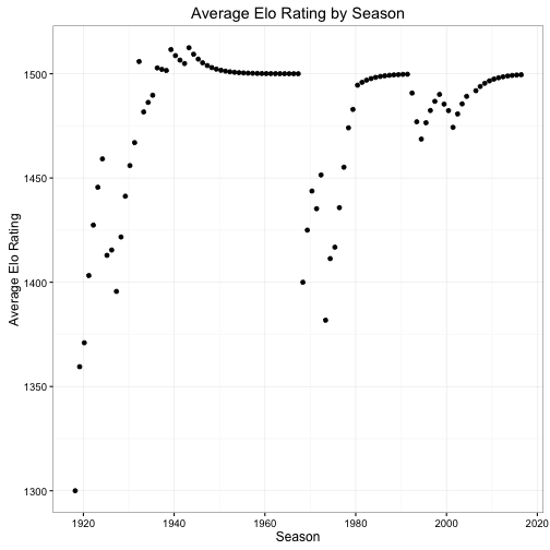
You’ll see that every time teams are added, the average Rating goes down, and slowly recovers to 1500 A few times the average goes above the target, this happens when low-ranked teams drop out of the league. By this method, we’re currently at 1499.54, but this will decrease next year as Las Vegas steps into the league.

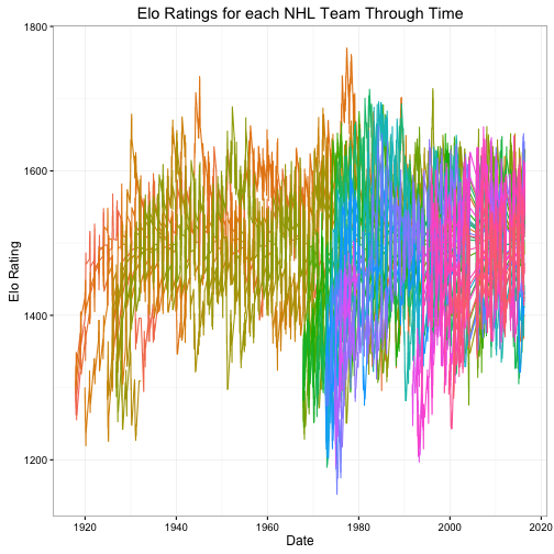
Here’s every team that has played in the league’s ratings over all time. I’ve dropped the legend because it takes up almost the entire plot canvas, as there are 48 teams in total. See this earlier post about handling teams that have moved or changed names in the past.

I plan to make a shiny app that I’ll link to, where you can investigate each team’s Elo history in a cleaner format. For the time being, here’s what one team looks like:

ggplot(data=elo_all_long[elo_all_long$Team == "Nashville.Predators",], 
        aes(x=Date, y=Rating)) +
     geom_line(colour='darkblue') +
     ggtitle("Elo Ratings for the Nashville Predators Through Time") +
     xlab("Date") +
     ylab("Elo Rating") +
     theme_bw() +
     theme(legend.position="none")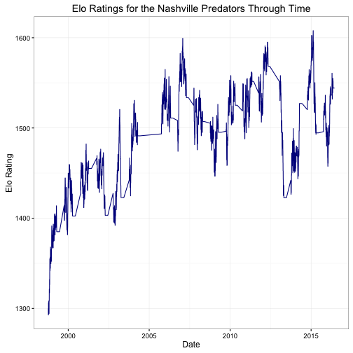

I’ll dig more into the Elo results next time.