Last time we created a distance matrix and a time matrix for use in TSP problems. We’re using a set of locations in the Ottawa, Ontario, Canada area, but any list of locations with addresses would work. Now we’ll work through getting optimized routes to visit each address once. We’ll optimize by distance, but we also generated a ‘time matrix’ and could run the TSP solver that way.

We’ll start this time by loading the data we saved last time:

distance_matrix<-readRDS("./_data/distance_matrix.RDS")
time_matrix<-readRDS("./_data/time_matrix.RDS")

Much of this post is informed by the vignette in the TSP package. There’s lots of great documentation in a more ‘tutorial’ type format than the official documentation in R vignettes.

We’ll start by making these matrices ‘TSP’ compatable objects.

ottawa_dm<-ATSP(distance_matrix)
ottawa_tm<-ATSP(time_matrix)

Note that we use the ATSP function. The matrices we’re feeding in aren’t symmetrical. It may take longer or be farther to go from point A to point B than it is to go from B to A. This could be due to traffic, one way streets, the number of left hand turns, etc.

We can look at a few properties of this ATSP class:

print(ottawa_dm)

## object of class 'ATSP'  (asymmetric TSP) 
## 46 cities (distance 'unknown')

head(labels(ottawa_dm))

## [1] "24 Sussex Dr, Ottawa, ON K1M 1M4, Canada"           
## [2] "2100 Cabot St, Ottawa, ON K1H 6K1, Canada"          
## [3] "2777 Cassels St, Ottawa, ON K2B 6N6, Canada"        
## [4] "1 Canal Ln, Ottawa, ON K1P 5P6, Canada"             
## [5] "55 Byward Market Square, Ottawa, ON K1N 9C3, Canada"
## [6] "2 Queen Elizabeth Dr, Ottawa, ON K2P 2H9, Canada"

We can also visualize a shaded matrix of the distances between objects:

image(ottawa_dm)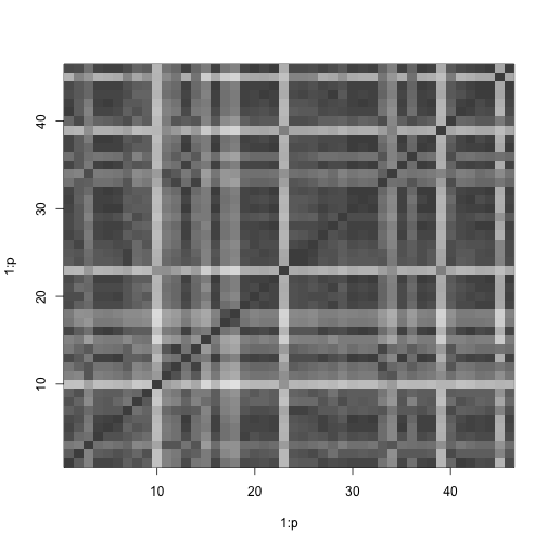

Let’s solve the TSP by each of the internal methods and see what minimum distance for each we get:

methods <- c("nearest_insertion", "farthest_insertion", "cheapest_insertion",
"arbitrary_insertion", "nn", "repetitive_nn", "two_opt")
dm_tours <- sapply(methods, FUN = function(m) solve_TSP(ottawa_dm, method = m), simplify = FALSE)
 
dotchart(sort(c(sapply(dm_tours, tour_length))))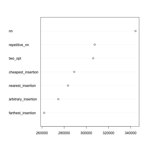

Some of the solver algorithms do much better than others at finding the optimal route. Remember, distances were given by the Google Distance Matrix API in meters, so we’re looking at a 330 km trip on the ‘worst’ solution, and closer to 260km on the good end.

How much better is that than a random tour? We can simulate a tour a few thousand times to get an estimate of the improvements that even a simple solver can give us:

distances<-list(rep(NA, 10000))
for(i in 1:10000){
    t<-sample(c(1:nrow(distance_matrix)))
    t<-c(t, t[1])
    d<-0
    for(j in 1:nrow(distance_matrix)){
        d<-d+distance_matrix[t[j],t[j+1]]
    }
    distances[i]<-d
}

This gives us a mean of 669.84389km, significantly longer than our ‘worst’ optimized route. One route came out as long as 774.348km, and the best ‘random’ route was 489.175km, which wasn’t terrible.

Concorde, Chained Lin-Kernighan (linkern) and other solvers can only do symmetric TSP. A function will convert our ATSP problem to a TSP for use with these advanced solvers. This function doubles each city, providing an ‘in’ and an ‘out’ city, with distance 0 between them (set as cheap = 0).

ottawa_dm_tsp<-reformulate_ATSP_as_TSP(ottawa_dm, cheap = 0)
ottawa_tm_tsp<-reformulate_ATSP_as_TSP(ottawa_tm, cheap = 0)
 
print(ottawa_dm_tsp)

## object of class 'TSP' 
## 92 cities (distance 'unknown')

We have to set the Concorde TSP path. It seems to work only with an abspath, no ~ involved.

concorde_path("/Users/pbulsink/concorde/TSP")

## found: concorde concorde.c concorde.o

We’ll try solve the TSP using concorde:

dm_tours$concorde <- solve_TSP(ottawa_dm_tsp, method="concorde", control = list(verbose=FALSE))

Similarly, we’ll reset the path to use the Chained Lin-Kernighan (linkern) method:

concorde_path("/Users/pbulsink/concorde/LINKERN")

## found: linkern linkern_fixed.c linkern_fixed.o linkern_path.c linkern_path.o linkern.a linkern.c linkern.o

dm_tours$linkern <- solve_TSP(ottawa_dm_tsp, method="linkern", control = list(verbose=FALSE))
dotchart(sort(c(sapply(dm_tours, tour_length))))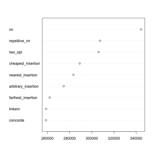

By looking at the bottom of the dot plot, we can see that the Lin-Kernighan and Concorde solvers provide the most optimal routes, and assorted substitution algorithms provide less qualified answers.

Next post we’ll discuss mapping the routes visually.

Remember that Concorde is licenced for academic use only, all other uses must be requested on the Concorde website.