Intro

No one likes to hear about their team having a back to back in any sport. With hockey, it’s the same.

Data

We’ll use some of the old scripts for loading and processing the hockey data. We’ll look at the last ten complete years of data (2006-2007 to 2016-2017).

#Load Data
nhl10<-readHockeyData(data_dir = "./_data/", nhl_year_list = c(2007:2017), playoffs = FALSE)
nhl10<-nhl10[nhl10$League == "NHL",]
nhl10<-nhl10[,c(1,2,3,4,5,6,11)]

A nasty set of ifs takes every game, and looks in the past few days to see if the home or away team was playing. If so, it sets the rest to 0 days rest (back to backs) up to 3 days (including > 3 days).

#Finding back to backs, rested, etc.
nhl10$HomeRest <- rep(3)
nhl10$VisitorRest <- rep(3)
 
for (g in seq_len(nrow(nhl10))){
  d<-nhl10[g,1]
  h<-nhl10[g,2]
  v<-nhl10[g,4]
 
  if(h %in% nhl10[nhl10[,1] == d - 1, 2] || h %in% nhl10[nhl10[,1] == d - 1, 4]){
    nhl10[g,8]<-0
  } else if(h %in% nhl10[nhl10[,1] == d - 2, 2] || h %in% nhl10[nhl10[,1] == d - 2, 4]){
    nhl10[g,8]<-1
  } else if(h %in% nhl10[nhl10[,1] == d - 3, 2] || h %in% nhl10[nhl10[,1] == d - 3, 4]){
    nhl10[g,8]<-2
  }
  if(v %in% nhl10[nhl10[,1] == d - 1, 2] || v %in% nhl10[nhl10[,1] == d - 1, 4]){
    nhl10[g,9]<-0
  } else if(v %in% nhl10[nhl10[,1] == d - 2, 2] || v %in% nhl10[nhl10[,1] == d - 2, 4]){
    nhl10[g,9]<-1
  } else if(v %in% nhl10[nhl10[,1] == d - 3, 2] || v %in% nhl10[nhl10[,1] == d - 3, 4]){
    nhl10[g,9]<-2
  }
}
 
nhl10$RestDifferent<-nhl10$HomeRest - nhl10$VisitorRest
nhl10$BinResult<-round(nhl10$Result)
nhl10$TriResult<-ifelse((nhl10$Result < 0.9 & nhl10$Result > 0.1), 0.5, nhl10$Result)

Analysis

We can see how the league typically schedules teams with a few quick ggplot graphics.

ggplot(data=nhl10) + 
  geom_histogram(aes(x=HomeRest, ..density..), fill='blue', alpha=0.3, binwidth = 1, center=0) +
  geom_histogram(aes(x=VisitorRest, ..density..), fill='red', alpha=0.3, binwidth = 1, center = 0) +
  ggtitle("Proportion of Days of Rest for Home(Blue) and Away (Red) Teams") + 
  xlab("Days of Rest") + 
  ylab("Proportion of Games") + 
  theme_bw()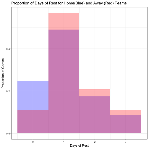

Clearly, the league doesn’t like to schedule back to back games for a team to have the second game on the road, as much as having the second game at home. This is accompanied by a similar reduction in rest days at home for 1-3 days.

Lets also look at the winning percentages for teams in each situation. To start, we’ll note that the total win percent for the home team in the past decade has been 54.65%. For each situation, the table is shown below

m<-matrix(rep(0.5), nrow = 4, ncol = 4)
rownames(m)<-c("Home.0", "Home.1", "Home.2", "Home.3+")
colnames(m)<-c("Visitor.0","Visitor.1","Visitor.2","Visitor.3+")
for(a in seq(1:4)){
  for(b in seq(1:4)){
    r<-mean(nhl10[nhl10$HomeRest == (a-1) & nhl10$VisitorRest == (b-1),"BinResult"])
    m[a,b] <- r
  }
}
pander(m)

  Visitor.0 Visitor.1 Visitor.2 Visitor.3+ ————- ———– ———– ———– ———— Home.0 0.5453 0.5941 0.5865 0.5116

Home.1 0.5435 0.5416 0.5521 0.5262

Home.2 0.4663 0.5281 0.5451 0.484

Home.3+ 0.4304 0.5662 0.559 0.5099

So, it looks like there’s some situations to avoid, such as being at home very rested against a busy visitor team. A win percentage of 43.04% is very low. That’s an interesting finding, but seems to hold some water as it’s happened 79 times in the past 10 years. Actually, none of these cases are infrequent, below is a table of the counts of each case.

m<-matrix(rep(0.5), nrow = 4, ncol = 4)
rownames(m)<-c("Home.0", "Home.1", "Home.2", "Home.3+")
colnames(m)<-c("Visitor.0","Visitor.1","Visitor.2","Visitor.3+")
for(a in seq(1:4)){
  for(b in seq(1:4)){
    r<-length(nhl10[nhl10$HomeRest == (a-1) & nhl10$VisitorRest == (b-1),"BinResult"])
    m[a,b] <- r
  }
}
pander(m)

  Visitor.0 Visitor.1 Visitor.2 Visitor.3+ ————- ———– ———– ———– ———— Home.0 629 1584 578 301

Home.1 506 4119 1065 458

Home.2 178 1032 798 188

Home.3+ 79 385 161 455

The above results look at overtime and shootout results with the same importance as regular wins. If we turn all overtime results into a set of {0, 0.5, 1}, representing home loss, overtime (either team winning), and home win, respectively, then we’ll get the following win chances:

m<-matrix(rep(0.5), nrow = 4, ncol = 4)
rownames(m)<-c("Home.0", "Home.1", "Home.2", "Home.3+")
colnames(m)<-c("Visitor.0","Visitor.1","Visitor.2","Visitor.3+")
for(a in seq(1:4)){
  for(b in seq(1:4)){
    r<-mean(nhl10[nhl10$HomeRest == (a-1) & nhl10$VisitorRest == (b-1),"TriResult"])
    m[a,b] <- r
  }
}
pander(m)

  Visitor.0 Visitor.1 Visitor.2 Visitor.3+ ————- ———– ———– ———– ———— Home.0 0.5644 0.5821 0.5779 0.5133

Home.1 0.5296 0.5426 0.5521 0.5295

Home.2 0.4831 0.5349 0.5476 0.4681

Home.3+ 0.4241 0.5403 0.5342 0.5099

The same effect is shown whether we account for overtime games or not.

Finally, we’ll look at expected goal differential, to see if there’s any insights in goal production by rest difference.

nhl10$GoalDiff <- nhl10$HomeGoals - nhl10$VisitorGoals
nhl10[nhl10$OTStatus != '', ]$GoalDiff <- 0
ggplot(data=nhl10, aes(x=RestDifferent, y=GoalDiff)) + 
  geom_point() +
  geom_smooth(method='lm') +
  ggtitle("Goal differential by Days Rest (+ favours home team)") + 
  xlab("Days of Rest") + 
  ylab("Goal Differential") + 
  theme_bw()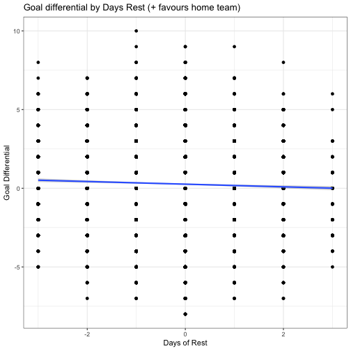

While technically that’s a negative line of best fit, the R^2 value for the fit is only 0.001458, which is functionally useless. Thus, no determination of the goal difference can be drawn from the amount of rest of the teams.

Conclusions

Everyone hates the thought of their favorite team playing back to back games. But, there’s no reason to fear. In fact, the data suggest that longer rests are more detrimental to a team’s performance.