Dixon-Coles and Hockey Data
Note: This is earlier work I did (last winter/spring) so some info may seem dated at time of posting. I’ve used data files current to then.
Last entry we did some data importing and cleaning of historical NHL data, from 2005 to present. This was in anticipation of performing simulation of games, by the Dixon-Coles method. Much of this entry is not my original work, I’ve used slightly modified versions of the code available from Jonas at the opisthokonta.com blog. I’ve mixed his optimized Dixon-Coles method and the time regression method which was a key part of Dixon and Coles’ paper.
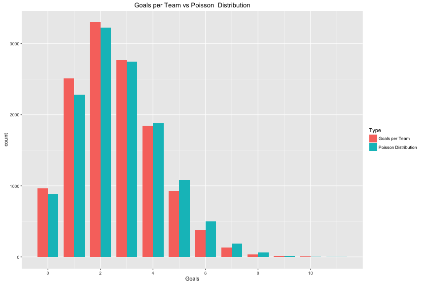
First, Dixon and Coles provide a method to increase the number of low-goal scoring games. A keen eye would notice that the goals scored is a bit biased ‘left’ compared to the actual Poisson curve:
The Dixon-Coles method for adjusting for low scoring games is the tau (τ) function, which we’ll use in a bit.
tau <- Vectorize(function(y1, y2, lambda, mu, rho) {
    if (y1 == 0 & y2 == 0) {
        return(1 - (lambda * mu * rho))
    } else if (y1 == 0 & y2 == 1) {
        return(1 + (lambda * rho))
    } else if (y1 == 1 & y2 == 0) {
        return(1 + (mu * rho))
    } else if (y1 == 1 & y2 == 1) {
        return(1 - rho)
    } else {
        return(1)
    }
})
This multiplied by the attack and defence rates of each team being modeled. The numbers become incredibly small, so Jonas adds the log of each instead:
DClogLik <- function(y1, y2, lambda, mu, rho = 0) {
    # rho=0, independence y1: home goals y2: away goals
    sum(log(tau(y1, y2, lambda, mu, rho)) + log(dpois(y1, lambda)) + log(dpois(y2,
        mu)))
}
These two functions are used below, when setting up the model to be optimized, and in the model itself. The reader is encouraged to visit the opisthokonta blog to learn more about what happens in these steps:
DCmodelData <- function(df) {

    team.names <- unique(c(levels(df$HomeTeam), levels(df$AwayTeam)))

    # attack, with sum-to-zero constraint home
    hm.a <- model.matrix(~HomeTeam - 1, data = df)
    hm.a[df$HomeTeam == team.names[length(team.names)], ] <- -1
    hm.a <- hm.a[, 1:(length(team.names) - 1)]

    # away
    am.a <- model.matrix(~AwayTeam - 1, data = df)
    am.a[df$AwayTeam == team.names[length(team.names)], ] <- -1
    am.a <- am.a[, 1:(length(team.names) - 1)]

    # defence, same as before
    hm.d <- model.matrix(~HomeTeam - 1, data = df)
    am.d <- model.matrix(~AwayTeam - 1, data = df)

    return(list(homeTeamDMa = hm.a, homeTeamDMd = hm.d, awayTeamDMa = am.a,
        awayTeamDMd = am.d, homeGoals = df$HG, awayGoals = df$AG, teams = team.names))
}

DCoptimFn <- function(params, DCm) {

    home.p <- params[1]
    rho.p <- params[2]

    nteams <- length(DCm$teams)
    attack.p <- matrix(params[3:(nteams + 1)], ncol = 1)  #one column less
    defence.p <- matrix(params[(nteams + 2):length(params)], ncol = 1)

    # need to multiply with the correct matrices
    lambda <- exp(DCm$homeTeamDMa %*% attack.p + DCm$awayTeamDMd %*% defence.p +
        home.p)
    mu <- exp(DCm$awayTeamDMa %*% attack.p + DCm$homeTeamDMd %*% defence.p)


    return(DClogLik(y1 = DCm$homeGoals, y2 = DCm$awayGoals, lambda, mu, rho.p) *
        -1)
}
I’ve taken the lines of code scattered through the opisthokonta blog posts and put them all together in two more easy-use functions:
doDCPrediction <- function(df) {
    # Get a useful data set
    dcm <- DCmodelData(df)
    nteams <- length(dcm$teams)

    # dummy fill parameters initial parameter estimates
    attack.params <- rep(0.03, times = nteams - 1)  # one less parameter
    defence.params <- rep(-0.2, times = nteams)
    home.param <- 0.1
    rho.init <- 0.1
    par.inits <- c(home.param, rho.init, attack.params, defence.params)

    # informative names skip the last team
    names(par.inits) <- c("HOME", "RHO", paste("Attack", dcm$teams[1:(nteams -
        1)], sep = "."), paste("Defence", dcm$teams, sep = "."))

    res <- optim(par = par.inits, fn = DCoptimFn, DCm = dcm, method = "BFGS")

    parameters <- res$par

    # compute last team attack parameter
    missing.attack <- sum(parameters[3:(nteams - 1)]) * -1

    # put it in the parameters vector
    parameters <- c(parameters[1:(nteams + 1)], missing.attack, parameters[(nteams +
        2):length(parameters)])
    names(parameters)[nteams + 2] <- paste("Attack.", dcm$teams[nteams], sep = "")

    # increase attack by one
    parameters[3:(nteams + 2)] <- parameters[3:(nteams + 2)] + 1

    # decrease defence by one
    parameters[(nteams + 3):length(parameters)] <- parameters[(nteams + 3):length(parameters)] -
        1

    res$par <- parameters
    return(res)

}
Use of this is to feed in the data into the doDCPrediction function, returning the res parameter object. This is a long calculation. We’ll use this result to simulate an actual game in the next post.
## Error in optim(par = par.inits, fn = DCoptimFn, DCm = dcm, method = "BFGS"): non-finite finite-difference value [2]The full 10 seasons took 302 seconds, while even just one season took 68 seconds. We haven’t even added in the promised time dependancy yet! WOW. Hopefully it’s a good model.
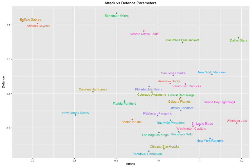
We’ll plot the Attack and Defence parameters for each team to se if there’s any correllation.
 The effect that time dependance has on the Poisson determination is weighting more recent games higher than older results. There are a few reasons why this matters, including the effect of short term hot and cold streaks, but also to account for how teams change over time (player quality changes due to age, players added and removed by trades, drafts, or retirement; changes in coaches or coaching style, etc). To add this to our method from above, we need to start with adding a weighting function based on ξ (xi):
DCweights <- function(dates, currentDate = Sys.Date(), xi = 0) {
    datediffs <- dates - as.Date(currentDate)
    datediffs <- as.numeric(datediffs * -1)
    w <- exp(-1 * xi * datediffs)
    w[datediffs <= 0] <- 0  #Future dates should have zero weights
    return(w)
}
We can see the effect this has by throwing the list of dates from our scores into the function, with different values of ξ.
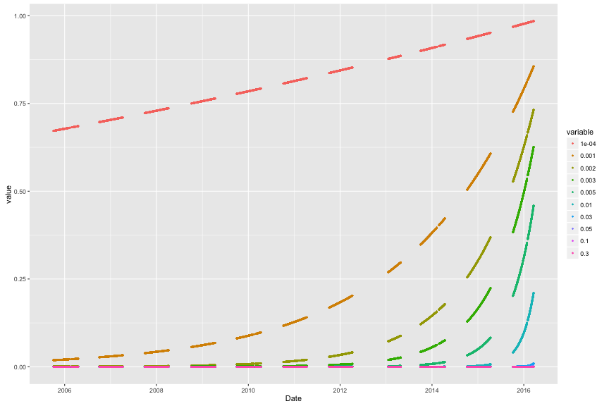
This graph shows the weight (0 to 1) of a game on a certain date. The lower the weight, the less it impacts the model’s optimization. The graph is choppy, because weights are given for games, there’s no games played in summer, and in 2012 there was a lockout (note the exta large gap).
While it might make sense to use a ξ value of 0.005 (focusing mostly on this season, somewhat on the last, but not much on seasons before that), evaulation of the performance of the model at each ξ value would be the best determiner of what to use. Again, we’ll look at that later.
With the weighting function available, we’ll modify the rest of the functions to use the weights:
DClogLik_w <- function(y1, y2, lambda, mu, rho = 0, weights = NULL) {
    # rho=0, independence y1 home goals y2 away goals
    loglik <- log(tau(y1, y2, lambda, mu, rho)) + log(dpois(y1, lambda)) + log(dpois(y2,
        mu))
    if (is.null(weights)) {
        return(sum(loglik))
    } else {
        return(sum(loglik * weights))
    }
}

DCmodelData_w <- function(df) {
    team.names <- unique(c(levels(df$HomeTeam), levels(df$AwayTeam)))

    # attack, with sum-to-zero constraint home
    hm.a <- model.matrix(~HomeTeam - 1, data = df)
    hm.a[df$HomeTeam == team.names[length(team.names)], ] <- -1
    hm.a <- hm.a[, 1:(length(team.names) - 1)]

    # away
    am.a <- model.matrix(~AwayTeam - 1, data = df)
    am.a[df$AwayTeam == team.names[length(team.names)], ] <- -1
    am.a <- am.a[, 1:(length(team.names) - 1)]

    # defence, same as before
    hm.d <- model.matrix(~HomeTeam - 1, data = df)
    am.d <- model.matrix(~AwayTeam - 1, data = df)

    return(list(homeTeamDMa = hm.a, homeTeamDMd = hm.d, awayTeamDMa = am.a,
        awayTeamDMd = am.d, homeGoals = df$HG, awayGoals = df$AG, dates = df$Date,
        teams = team.names))
}

DCoptimFn_w <- function(params, DCm, xi = 0) {
    home.p <- params[1]
    rho.p <- params[2]

    nteams <- length(DCm$teams)
    attack.p <- matrix(params[3:(nteams + 1)], ncol = 1)  #one column less
    defence.p <- matrix(params[(nteams + 2):length(params)], ncol = 1)

    # need to multiply with the correct matrices
    lambda <- exp(DCm$homeTeamDMa %*% attack.p + DCm$awayTeamDMd %*% defence.p +
        home.p)
    mu <- exp(DCm$awayTeamDMa %*% attack.p + DCm$homeTeamDMd %*% defence.p)

    w <- DCweights(DCm$dates, xi = xi)
    return(DClogLik_w(y1 = DCm$homeGoals, y2 = DCm$awayGoals, lambda, mu, rho.p,
        w) * -1)
}

doDCPrediction_w <- function(df, xi = 0) {
    # Get a useful data set
    dcm <- DCmodelData_w(df)
    nteams <- length(dcm$teams)

    # dummy fill parameters initial parameter estimates
    attack.params <- rep(0.1, times = nteams - 1)  # one less parameter
    defence.params <- rep(-0.8, times = nteams)
    home.param <- 0.06
    rho.init <- 0.03
    par.inits <- c(home.param, rho.init, attack.params, defence.params)

    # informative names skip the last team
    names(par.inits) <- c("HOME", "RHO", paste("Attack", dcm$teams[1:(nteams -
        1)], sep = "."), paste("Defence", dcm$teams, sep = "."))

    res <- optim(par = par.inits, fn = DCoptimFn_w, DCm = dcm, xi = xi, method = "BFGS",
        hessian = FALSE)

    parameters <- res$par

    # compute last team attack parameter
    missing.attack <- sum(parameters[3:(nteams + 1)]) * -1

    # put it in the parameters vector
    parameters <- c(parameters[1:(nteams + 1)], missing.attack, parameters[(nteams +
        2):length(parameters)])
    names(parameters)[nteams + 2] <- paste("Attack.", dcm$teams[nteams], sep = "")

    # increase attack by one
    parameters[3:(nteams + 2)] <- parameters[3:(nteams + 2)] + 1

    # decrease defence by one
    parameters[(nteams + 3):length(parameters)] <- parameters[(nteams + 3):length(parameters)] -
        1

    res$par <- parameters
    return(res)
}
Remaking those functions took a lot of space, but only a few lines changed. We multiply the log likelyhood function by weights, and the remainder is to bring the calculated weights from the user through the model.
Running it again, we get 10 seasons taking 547 seconds, and one season 40 seconds. We could optimize that futher if we wanted (eg. drop data for weight of less than some amount), but fortunately we only have to run this once to start predicting all sorts of results.
We’ll plot the Attack and Defence parameters for each team to se if there’s any correllation.

library(knitr)
kable(team_params)| Team | Attack | Defence |
|---|---|---|
| Philadelphia Flyers | 0.9788685 | -0.0790512 |
| Vancouver Canucks | 1.0653285 | -0.0716426 |
| San Jose Sharks | 1.0363260 | -0.0470196 |
| Montreal Canadiens | 0.9781757 | -0.2675670 |
| Winnipeg Jets | 1.1885145 | -0.1861203 |
| Columbus Blue Jackets | 1.0588779 | 0.0488788 |
| Chicago Blackhawks | 1.0142106 | -0.2610679 |
| Boston Bruins | 0.9381271 | -0.1748817 |
| Calgary Flames | 1.0520708 | -0.1149490 |
| Colorado Avalanche | 0.9855419 | -0.0955395 |
| Ottawa Senators | 1.0544292 | -0.1488981 |
| New Jersey Devils | 0.8025751 | -0.1623552 |
| Anaheim Ducks | 1.0291692 | -0.0705651 |
| New York Rangers | 1.1246283 | -0.2301985 |
| Florida Panthers | 0.9200872 | -0.1212742 |
| New York Islanders | 1.1289564 | -0.0438022 |
| Los Angeles Kings | 1.0024739 | -0.2126434 |
| Washington Capitals | 1.0839849 | -0.1946443 |
| Buffalo Sabres | 0.6755308 | 0.1105787 |
| Minnesota Wild | 1.0494299 | -0.2112040 |
| Dallas Stars | 1.1928880 | 0.0639135 |
| Carolina Hurricanes | 0.8444117 | -0.0946161 |
| Pittsburgh Penguins | 0.9986188 | -0.1643924 |
| Edmonton Oilers | 0.9010637 | 0.1349262 |
| Toronto Maple Leafs | 0.9660961 | 0.0829082 |
| St. Louis Blues | 1.0989753 | -0.1934415 |
| Detroit Red Wings | 1.0542852 | -0.1113708 |
| Nashville Predators | 1.0303242 | -0.1773239 |
| Tampa Bay Lightning | 1.1833470 | -0.1245115 |
| Arizona Coyotes | 0.7119971 | 0.1045630 |
There’s another way of generating the teams strengths, and this is wicked fast. Again, this is based on opisthokonta and from Martin Eastwood and the pena.lt/y blog. This method is slightly lsess accurate, and doesn’t do time dependance (yet) but is fast enough and simple enough to cut it.
I’ll write it out here in a fully implemeneted function, but in essance, a linear fit of Goals as predicted by the combination of Home (for any given game), Team (whichever team we focus on) and Away (for any given game). This gives us back a list of parameters in the form of a ‘Home’ strength, and Team[nhlteam] and Opponent[nhlteam] strengths. Those are fed back into the ‘fitted’ function which provides us with the expected goals for each game, provided as a list of home goals followed by away goals. When those are compared to the actual goals in the DCoptimRhoFn, we get a value for rho, the low-scoring enhancer. Lambda and mu are extracted using the predict function. The remainder of the score prediction code we have works the same from this point on, but I’ve included some of it to get a prediction value out.
doFastFit <- function(df) {
    df.indep <- data.frame(Team = as.factor(c(as.character(df$HomeTeam), as.character(df$AwayTeam))),
        Opponent = as.factor(c(as.character(df$AwayTeam), as.character(df$HomeTeam))),
        Goals = c(df$HG, df$AG), Home = c(rep(1, dim(df)[1]), rep(0, dim(df)[1])))
    m <- glm(Goals ~ Home + Team + Opponent, data = df.indep, family = poisson())
    return(m)
}

doFastDC <- function(m, df) {
    expected <- fitted(m)
    home.expected <- expected[1:nrow(df)]
    away.expected <- expected[(nrow(df) + 1):(nrow(df) * 2)]

    DCoptimRhoFn.fast <- function(par) {
        rho <- par[1]
        DClogLik(df$HG, df$AG, home.expected, away.expected, rho)
    }

    res <- optim(par = c(0.1), fn = DCoptimRhoFn.fast, control = list(fnscale = -1),
        method = "BFGS")
    return(res)
}

fastDCPredict <- function(m, res, home, away, maxgoal = 7) {
    # Expected goals home
    lambda <- predict(m, data.frame(Home = 1, Team = home, Opponent = away),
        type = "response")

    # Expected goals away
    mu <- predict(m, data.frame(Home = 0, Team = away, Opponent = home), type = "response")

    probability_matrix <- dpois(0:maxgoal, lambda) %*% t(dpois(0:maxgoal, mu))

    scaling_matrix <- matrix(tau(c(0, 1, 0, 1), c(0, 0, 1, 1), lambda, mu, res$par),
        nrow = 2)
    probability_matrix[1:2, 1:2] <- probability_matrix[1:2, 1:2] * scaling_matrix

    HomeWinProbability <- sum(probability_matrix[lower.tri(probability_matrix)])
    DrawProbability <- sum(diag(probability_matrix))
    AwayWinProbability <- sum(probability_matrix[upper.tri(probability_matrix)])

    return(c(HomeWinProbability, DrawProbability, AwayWinProbability))
}

t <- proc.time()
mAll <- doFastFit(nhl_all)
resAll <- doFastDC(mAll, nhl_all)
tFast <- proc.time() - t
So, for all the data, that provides us with a fitting in 3 seconds, compared to 547 seconds for the above method. We’ll continue to use this method for speed in later work as we predict results for some games!